Predictive Maintenance for Crushing Plants - Part 2

In part 2 of this two-part blog series, we have presented a method for predictive maintenance on machines in a cone-crushing plant using machine learning and deep learning techniques. In part 1, we showed how we can use data from the wear profiles of the cone crusher liners to optimize the time to replace the wear parts and to detect any anomalies in the wear patterns. In part 2, we discussed how we can collect and preprocess other types of data from the cone crusher, such as temperature, pressure, and vibration, and apply similar models to detect anomalies in the function of the plant. Our method can help improve the efficiency, reliability, and safety of the cone-crushing plant, as well as reduce operational costs and environmental impacts.

Why collect more data?

Deep learning models are known for their need for large amounts of data. Without sufficient data, these models tend to overfit the training data and do not generalize well in production. Moreover, the data must be informative enough for the specific task at hand. For instance, if we want to build a model to predict housing prices, and our data only includes the total square footage and the number of bathrooms, our model will not perform well on real data without additional features like location and age of the house.

Detecting different and varied Faults and Anomalies

in the context of a cone crusher, different faults and anomalies will manifest in different parts of the machine. For example, a misalignment in the main shaft will alter the wear profile of the cone mantle, while a suboptimal lubrication system will result in higher oil temperature and power draw due to increased friction.

Real-Time Anomaly Detection for Predictive Maintenance

Real-time data collection and processing can significantly improve the efficiency of predictive maintenance. Measurements such as the closed side setting (CSS) can only be taken when the machine is not running. However, other types of data like vibration and temperature can be collected in real-time. Therefore, a model that can process this real-time data will allow us to detect anomalies during production and prevent catastrophic faults. This highlights the importance of collecting and utilizing a diverse range of data for predictive maintenance.

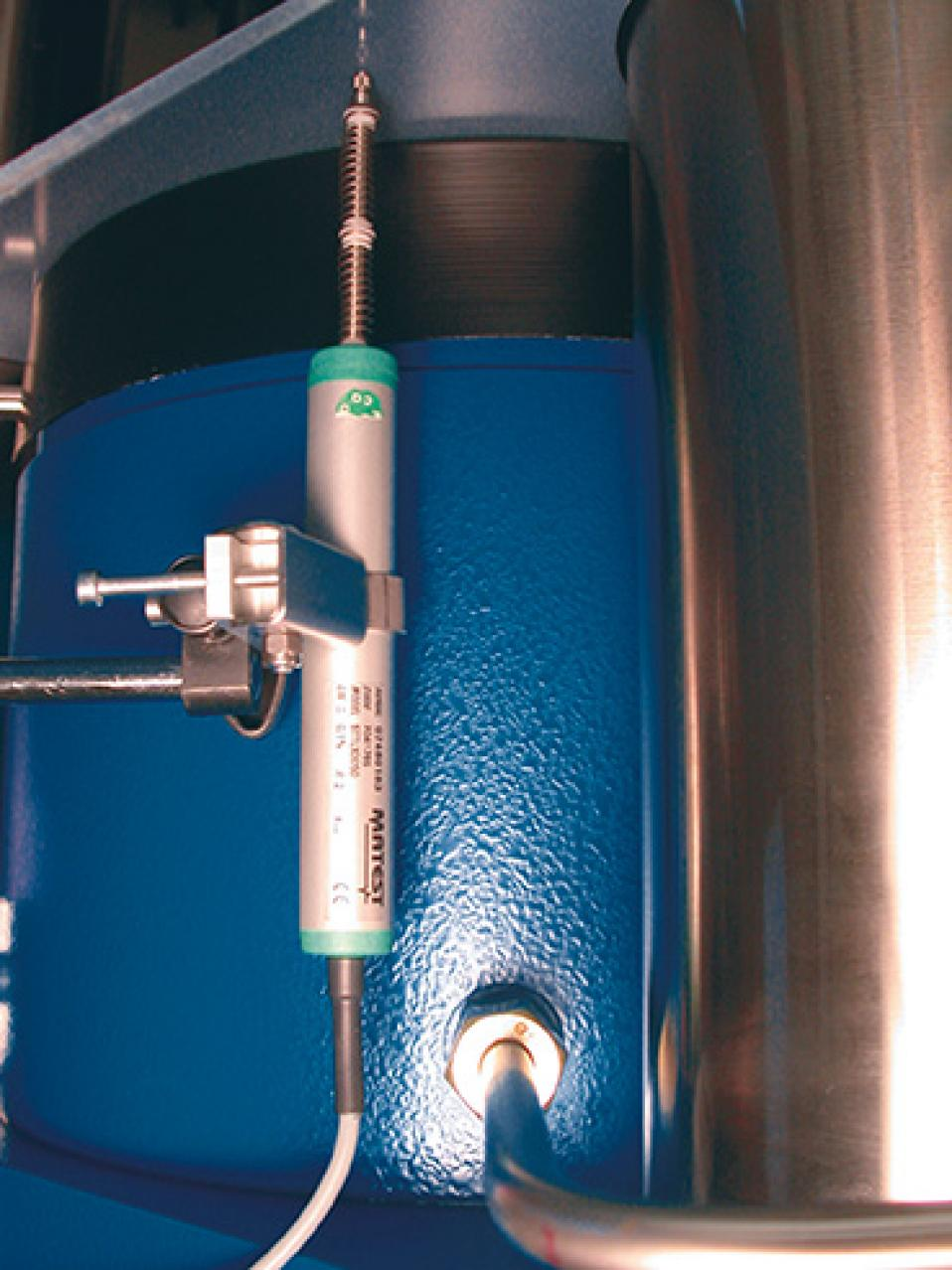
Sensors for cone crusher

To monitor the performance of the cone crusher in real time, we also need to install various sensors that can collect and transmit data about the machine’s condition. The sensors relevant to the cone crusher are:

1. Vibration sensors

2. Acoustic sensors

3. Cameras

4. lidar sensors

5. Oil flow sensors

6. Oil temperature sensors

7. Power usage sensors

Data collection

From the readings from these sensors, we will be collecting data that will give us an insight into the functioning of the cone crusher. We will discuss how each sensor might help build the feature vector for the representation of the state of the machine.

• Vibration sensors: These will monitor the frequency pattern of the machine and detect any changes that indicate a fault or a developing fault.

• Acoustic sensors: These will record the sound of the motor and other parts of the machine and help us identify any abnormal noises that signal a problem.

• Cameras: These will capture images of the output material and analyze its shape and cubicity, which are measures of the quality and efficiency of the crushing process.

• Oil flow sensors: These will ensure that the lubrication system is working properly and that the oil is circulating smoothly and sufficiently to prevent friction and damage to the machine parts.

• Oil temperature sensors: These will measure the temperature of the oil and alert us if it goes above or below the optimal range, which could affect the viscosity and performance of the lubrication system.

• Power usage sensors: These will track the amount of electricity that the machine consumes and help us identify any spikes or drops that could indicate a fault or a potential failure.

• Lidar sensors: These sensors will be used to measure the closed side setting (CSS) of the cone crusher. Since these readings can only be taken when the machine is not running, we will have to make an assumption that the cone mantle wears linearly during a production session. This will allow us to extrapolate and have a CSS reading for each time step.

Data preprocessing

Data preprocessing is an important step in predictive maintenance, as it can improve the quality and reliability of the data collected from different sensors. In this section, we will describe how we preprocess the data from each sensor individually, and what features we extract from them. We will use a 15-minute window for each sensor, as it is a common practice in predictive maintenance.

vibration sensors

Given the outdoor setting of our machine monitoring, the data from vibration sensors is likely to contain a significant amount of noise. To address this, we can apply various preprocessing techniques:

1. Denoising: We can utilize filtering and smoothing methods to eliminate most of the noise from vibration signals. Numerous open-source Python libraries offer implementations of these methods.

2. Find condition indicators: Once we have clean data, the next step is to extract condition indicators from the raw data. These indicators can be derived in several ways:

3. Signal-based Indicators: Simple statistical measures like mean and standard deviation over the period can serve as basic indicators.

4. Complex Signal Analysis: More sophisticated analysis can involve examining the frequency of the peak magnitude in a signal spectrum or a statistical moment describing changes in the spectrum over time.

5. Model-based Analysis: This involves estimating a state space model using the data and then analyzing the maximum eigenvalue.

6. Hybrid Approaches: These approaches combine both model-based and signal-based methods. For instance, we can use the signal to estimate a dynamic model, simulate the dynamic model to compute a residual signal, and then perform statistical analysis on the residual.

Acoustic sensors:

Acoustic sensors, like vibration sensors, are likely to capture a significant amount of noise due to the outdoor environment of our machine monitoring. However, traditional denoising methods may not be effective here as they might not be able to distinguish the useful sound from the noise.

In deep learning, mel spectrograms are commonly used as representations of sound for input to models. A mel spectrogram applies a frequency-domain filter bank to time-windowed audio signals. These spectrograms can then be processed with convolutional layers in our model, providing a robust method for handling the noisy data from acoustic sensors.

Cameras for cubicity/sphericity measurement:

Using cameras for cubicity measurement presents a complex challenge in our input vector. While there are third-party software solutions available for estimating the shape of our output feed, these require detailed study to ensure their effectiveness. Yang, J., & Chen, S. (2016) proposed some promising methods that might apply to our situation.

However, if these methods prove insufficient, we will develop a novel deep computer vision-based system to estimate the cubicity of the three different products. This system would provide three floating-point values indicating the percentage of cubic material in each product. Given that cubicity doesn’t change rapidly, we can afford to take this reading once per window. This approach allows us to balance the need for accurate data with the practicalities of data collection.

An online detection system for aggregate sizes and shapes based on digital image processing

Oil flow and oil temperature: The measurements from oil flow and temperature sensors are straightforward yet crucial. We would simply need to take the mean of the readings over each time window. These measurements provide vital information about the lubrication and cooling status of the machine.

Power usage sensors: Power usage sensors present a different challenge. The power draw of the cone crusher is highly volatile, depending on factors such as the input feed size and the type of material. Therefore, we need to clean and smooth the data to prepare it for analysis. This process, along with finding condition indicators, will be particularly useful here, given the volatility similar to that of vibration frequencies.

Feature vector

In the diagram above, we show how we can construct the feature vector using the readings from the sensors. The Convolutional Neural Network (CNN) models included in our approach represent the preprocessing required for the mel spectrograms and the images received from the cameras for cubicity measurements. These models will be pre-trained to output appropriate latent representations as needed. This process forms the basis of our feature construction, enabling us to capture and utilize the most relevant information from our sensor data.

Model architecture

Our model architecture for the wear parts of the cone crusher will employ an autoencoder with Long Short-Term Memory (LSTM) layers for encoding and decoding the input data. The primary objective of this model is to reconstruct the feature vector that represents the healthy functioning of the cone crusher. It’s important to note that the specific parameters of the model, such as the number of LSTM cells, the number of nodes in the fully connected layers, and the output shape, are only representative at this stage. We anticipate that some experimentation will be necessary to determine the optimal model architecture.

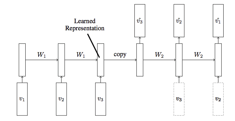
An LSTM autoencoder is a type of recurrent neural network used for sequence-to-sequence problems. It consists of two main components: an encoder and a decoder.

1. Encoder: The encoder processes the input sequence and compresses it into a fixed-length vector representation, also known as the “context vector” or “latent vector”. This is done through several LSTM layers. In the diagram, the encoder consists of two LSTM layers with 16 and 96 units respectively.

2. Decoder: The decoder takes the context vector and generates the output sequence. It also consists of several LSTM layers. In the diagram, the decoder has two LSTM layers with 96 and 16 units respectively.

The goal of the LSTM autoencoder is to reconstruct the input sequence as accurately as possible. This is achieved by minimizing the difference between the input sequence and the output sequence during training. The LSTM autoencoder learns to capture the most important features of the input sequence in the context vector, which can be used for various tasks such as anomaly detection, dimensionality reduction, and time series forecasting.

Model Training:

Mean Squared Error (MSE): This is calculated by taking the difference between the predicted output (ŷ) and the actual output (y) for each data point (i), squaring it, and then averaging these squared differences over all data points (n).

Our loss function will be the Mean Squared Error between the predicted value and the true value. Note the true value in this case will be just the input sequence since that's what the autoencoder has to reconstruct.

Optimization:

During the training process, the model tries to minimize this MSE loss. This is done using an optimization algorithm, typically gradient descent, which iteratively adjusts the model’s parameters to reduce the MSE.

note: In the context of an autoencoder, the MSE is often referred to as the “reconstruction loss”. This is because the autoencoder tries to reconstruct the input data from the encoded representation, and the MSE measures how well the reconstructed data matches the original input data.

Model evaluation:

Once the model has been sufficiently trained, which is determined by observing that the loss value no longer decreases despite further training, we can evaluate its performance on the test set. This is data that the model has not been trained on, providing a true test of its generalization ability.

loss on normal test data

For well-trained models, the reconstruction loss on normal test data is typically low. For instance, in most examples here in the test set, the reconstruction loss is center around a value like 0.02.

The loss plot on the data for anomalies will look a little different from the data that we already trained on, the distribution will be centered around a significantly higher reconstruction loss since the autoencoder hasn’t been trained on this data.However, when the model encounters anomalous data, which it hasn’t been trained on, the distribution of the reconstruction loss will be different. It will likely be centered around a significantly higher value, reflecting the model’s struggle to accurately reconstruct these unfamiliar data points.

By plotting the reconstruction loss for normal and anomalous data together, we can clearly see the difference between them. This allows us to establish a threshold for classification between normal data and anomalies, enhancing our model’s ability to detect unusual patterns in the data.

Anomaly detection during production

During production, we can utilize this model to detect any anomalies in the functioning of the cone crusher. This is achieved by logging all sensor data for the same time frame that the model was trained on and feeding this data into the autoencoder.

We previously established a threshold during the evaluation phase to categorize data as normal or anomalous. If the reconstruction loss exceeds this threshold, we tag the data point as an anomaly. Subsequent steps, such as triggering an alarm or sending a notification, can then be taken based on this anomaly detection.

It’s also crucial to continually log sensor data and periodically retrain our pre-existing autoencoder. This ongoing training process helps to improve the model’s accuracy over time, ensuring it remains effective as the machine’s operating conditions change.

Conclusion

In this post, we discussed how we use sensor data to detect anomalies in a cone crusher in a stone-crushing plant. We looked at the different sensors that we need to collect the data and then discussed how to preprocess them to construct a feature vector that can be used as input to an LSTM autoencoder. We saw how we can train the model and how to come up with a threshold to categorize an anomaly from the normal functioning of the cone crusher.

Smart Monitoring and Predictive Maintenance in Stone Crushing Plant using LSTM Autoencoders- part 1

In this article, we will delve into the application of Long Short-Term Memory (LSTM) Autoencoders for predictive maintenance in a stone crushing plant. If you’re new to this topic, I recommend reviewing my previous articles where I’ve discussed the working principles of a stone crushing plant, the operational challenges it faces, and the necessary sensors for applying machine learning algorithms. This will provide a better context for the information presented here.

Our primary focus will be on LSTM Autoencoders, a type of recurrent neural network that is particularly effective at learning from time series data. This makes them an ideal choice for analyzing sensor data for anomaly detection and predictive maintenance in the context of a stone crushing plant.

While we will touch upon the use of a plant dashboard for real-time monitoring, the main emphasis will be on the application and benefits of LSTM Autoencoders in this setting.

Why make a Smart Plant Dashboard?

Using a sensor-informed smart dashboard to monitor an industrial plant offers several advantages:

1. Real-Time Monitoring: Sensors provide real-time data on various parameters of the plant’s operations. This allows for immediate detection of any anomalies or deviations from the norm.

2. Efficiency: A smart dashboard provides a centralized view of all operational aspects of the plant. This makes it easier to identify areas where efficiency can be improved.

3. Safety: Continuous monitoring of the plant’s operations can help in identifying potential safety hazards. This can contribute to creating a safer working environment.

4. Human Analysis: The data presented on the dashboard can be analyzed by plant operators and managers. This human analysis can provide insights that automated systems might miss, and allows for more informed decision-making.

Edge-to-Cloud IIoT for Condition Monitoring in Manufacturing Systems with Ubiquitous Smart Sensors

In Li z et. al. They use MEM sensors to take vibration readings from an electronic component insertion machine. This is then passed to an edge layer and then relayed and stored in a centralized cloud service. In this way, data can be collected, stored, and eventually displayed for monitoring.

This is an example of a plant dashboard that is updated in real-time. All the readings are displayed in one place in a way where it is easy to compare readings between different machines. There is also some time series data, using which we can get an idea of the progression of the readings.

Predictive maintenance

The data collected from the plant can indeed be leveraged for predictive maintenance. However, it’s crucial to note that this data will likely be highly imbalanced due to the infrequency of machine failures. This imbalance necessitates the use of unsupervised machine learning methods, as we will predominantly be dealing with unlabeled data.

There are various methodologies available for detecting anomalies in machine function. Until now, our perspective has been plant-centric, considering the entire plant when addressing the issue. However, for predictive maintenance, it would be beneficial to shift our focus to individual machines. This is because each machine operates on a largely independent maintenance schedule.

In essence, a more granular, machine-level approach could enhance the effectiveness of our predictive maintenance efforts. Remember, the key to successful predictive maintenance lies in the quality of the data collected and the appropriateness of the analytical methods employed.

Cone crusher

The Cone crusher is the most critical machine in the plant. This machine requires regular maintenance, and it’s important to note that its spare parts can be quite costly. We have previously discussed the working principle of the cone crusher and the various components involved. It’s essential to understand these aspects to effectively manage and maintain the machine.

Wear profile estimation for wear parts

The longevity of the cone crusher liner is a crucial aspect of a plant’s operation and profitability. Typically, our cone crusher liner is replaced every 30,000 tons. However, this frequency can vary depending on the type of material being crushed. For instance, when crushing limestone, the replacement may be required 4-5 times more frequently.

The Remaining Useful Life (RUL) of this component is of paramount importance. Given that it’s a wear part, monitoring the rate of wear is essential to detect any deviations from the normal functioning of the cone crusher.

To measure the wear of the cone mantel and liner, we don’t necessarily need complex algorithms. The wear of the liner will naturally increase as the cone crusher continues to be used for production. The key is to analyze the rate of this wear and establish thresholds to identify any outlier values. This simple yet effective approach ensures the optimal functioning and longevity of the cone crusher.

Data collection

Firstly, we would measure the closed-side setting (CSS) and the open-side setting (OSS) for the cone mantel and liner. These settings indicate the distance between the mantle and liner at the bottom and the top of the cone crusher, respectively. We would also measure the position of the main shaft using the hydraulic system. Secondly, since the OSS and CSS measurement can only be done before and after a session, we would not be able to have real-time wear measurements.

Establish baselines:

We first need to measure the baseline, that is, the case where there is 0% wear. We will do this by doing the following when we install a new cone mantel and liner set.

• Raise the main shaft to its highest and measure the CSS. This is CSS with 0% wear.

• Use the cone mantel and liner with the needed CSS required.

• As we keep using the worn parts, after a session, repeat step 1. Raise the main shaft to it’s highest and measure the CSS.

• There will come a point where we will be using the cone mantel and liner with main shaft at it’s highest. As we keep using the machine, we will no longer be able to achieve the required CSS even wit the main shaft at it’s highest. At this point, we can call this 100% wear.

Logging Time: Given that the CSS measurement can only be conducted after a session, our readings will be captured in discrete time steps.

Production Logging: An alternative approach could be to log the number of tons produced instead of the number of production hours. This is because we tend to have more empirical data on the former

Data processing

To analyze the wear of the cone mantel and liner, we need to process the data we have collected from the readings. Instead of the absolute wear values at different time points, we are more interested in the rate of change of the wear over time.

• Calculate rate of change: We can estimate the rate of change by taking the difference between two consecutive wear readings and dividing it by the time interval between them. We can use either the number of hours or the number of tons produced as the time unit.

• Account for irregular time steps: Since the wear readings are not taken at regular intervals, we need to adjust the rate of change calculation accordingly. The time interval should reflect the actual duration between two readings.
  

Plotting

This plot shows the expected wear pattern of the mantle and liner. Initially, there is a high wear rate due to the break-in period, followed by a steady wear rate as the components operate normally. Finally, as the mantle and liner approach failure, the wear rate increases rapidly.

Predicting the time for replacement and repair

Once we have the time series data of the wear and the rate of wear measurements, we can employ a standard Long Short-Term Memory (LSTM) model to predict when the wear will exceed the 100% mark. The inputs to this model would be the wear percentage and the rate of change measured after every session, while the output would be the number of hours of production. This approach allows us to proactively schedule maintenance and replacement, thereby enhancing the efficiency and longevity of the cone crusher.

• The process begins with an LSTM (Long Short-Term Memory) cell, which is depicted on the left.

• The input data is then passed through the LSTM model, which consists of multiple LSTM cells. These cells are represented as ‘A’.

• At each step, the model estimates the time of repair.

• As more data is processed, these estimates are continually updated, leading to increasingly accurate predictions over time.

In this equation:

• Tons Left: represents the predicted number of tons left for the cone mantel and liner.

• LSTM(X): represents the LSTM (Long Short-Term Memory) model as a function that takes an input X.

• Current Cumulative Tons Produced: represents the current cumulative tons produced.
  

Anomaly detection using autoencoders The wear pattern of cone crusher parts can indeed vary based on several factors. For instance, setting the Closed Side Setting (CSS) too low can accelerate and possibly uneven the wear rate. Other potential causes for irregular wear patterns could be a fault in the motor or misalignment of the main shaft, among others. It’s crucial to detect these anomalies early to prevent further damage to the machine.

To this end, anomaly detection techniques in machine learning and deep learning can be employed. These techniques can help identify wear patterns that deviate from the norm, indicating potential issues with the machine’s operation. By leveraging these advanced methods, we can ensure the health and longevity of the machine, thereby enhancing its efficiency and productivity.

The image depicts a cone mantel that has worn unevenly, with more wear visible at the top and bottom, while the middle part exhibits less wear. This uneven wear pattern can lead to inefficient usage of the mantel, as it does not fully utilize the lifespan of the part. It’s crucial to monitor and address such wear patterns to ensure optimal performance and longevity of the cone crusher.

LSTM Autoencoders

The paragraph describes an LSTM (Long Short-Term Memory) autoencoder, which is a type of recurrent neural network used for sequence data. In this model:

• W1 represents the encoder, which learns a representation of the sequence in a latent space.

• W2 represents the decoder, which reconstructs the data one by one.

• v1, v2, v3 are the data points in the input sequence.

The encoder takes the input sequence and compresses it into a latent space representation. This representation is then passed to the decoder, which reconstructs the data sequentially. The first output should be v3, the second output should be v2, and so on. This process allows the model to capture the temporal dependencies in the data and reconstruct the sequence accurately. Data

As previously discussed, the data collection process will yield wear and rate of change of wear at irregular intervals. For instance, sometimes the machine may run for an hour, and sometimes for six hours. To create a consistent dataset, we can distribute the wear evenly across the hours of operation.

For example, if the cone crusher operates for six hours and incurs 6% wear, we can assume that the wear is distributed linearly across those six hours, attributing 1% wear to each hour.

We believe a window size of 64 hours is reasonable, as this is the maximum duration the cone crusher can operate over a four-day period. However, this window size could be adjusted if necessary.

Therefore, the input size would be (64,1), with these 64 values fed sequentially to the encoder. The output sequence would also be (64,1). As this is a reconstruction, both of these vectors would be identical. This approach allows us to create a regularized dataset from irregular time intervals, enhancing the effectiveness of our predictive model.

Training Process Loss function: The loss function will be MSE(mean squared error) between the input and the output data. This can also be called reconstruction error.

• ‘Yi’ represents the output of the decoder for the given time steps.

• ‘y^’ stands for the true value.

• The difference between these values is squared, summed over all examples in the batch, and then divided by the number of examples. This forms the basis of the mean squared error used as the reconstruction loss.

• Unlike typical LSTM applications for next-word generation, where the output sequence is shifted one timestep to the right, our goal here is to reconstruct the sequence.

The two graphs illustrate the performance of the model under normal and abnormal conditions for the cone crusher. The red line represents the actual data, while the blue line represents the predicted data.

Under normal conditions, the model’s predictions closely align with the actual data, indicating the healthy functioning of the cone crusher. However, under abnormal conditions, which could suggest a potential fault in the machine, the model’s predictions deviate significantly from the actual data. This is expected and desirable, as the model isn’t trained on such sequences and therefore, the loss is higher.

Loss on normal test data

As you can see there is a discrepancy in the loss when testing on normal data and anomaly data. The loss for the normal data is much less, hovering around 0.02, but for the anomaly data, the loss is around 0.9.

This discrepancy in the loss under abnormal conditions is precisely what we leverage for anomaly detection. A higher loss indicates a deviation from the normal operational patterns, thus signaling a potential anomaly or fault in the machine. This approach allows us to proactively identify issues and perform necessary maintenance or repairs.

Setting a threshold for anomaly detection is crucial. If the loss exceeds this threshold, we classify it as an anomaly. Conversely, if the loss is below the threshold, we classify it as normal data.

One approach could be to prioritize capturing all anomalies, even at the risk of occasionally misclassifying normal data as anomalous. This strategy prioritizes the detection of potential faults, ensuring the efficient operation and maintenance of the machine. However, it’s important to strike a balance to avoid excessive false positives, which could lead to unnecessary inspections and interventions.

Conclusion

In this blog post, we explored how to use sensor data from a stone crushing plant to optimize its performance. We applied machine learning and deep learning techniques to predict the optimal time to replace the wear parts in a cone crusher. We also detected anomalies in the wear profiles of the parts over time, which can help us identify potential faults and damages in the machine. In the next part, we will examine how to collect and analyze other types of data from the machine that can indicate different kinds of problems. This way, we can improve the efficiency and reliability of the stone crushing plant.

Stone Crushing Plant Sensor Suite

In this post, we will discuss the considerations for sensors in a stone crushing plant. It is advised that you go through 'Anatomy of a Stone Crushing Plant' and 'Operating Challenges in a Stone Crushing Plant' before reading further since that will give you all the context that you need about this post. There we discuss how a crushing plant works, what are the common operating challenges and the possible solutions to them. Selections made for the sensors in this post are considering the applications of machine learning and deep learning models that we will train and use in order to solve these operating challenges.

Why do we need sensors?

Machine learning models work by training on a dataset and hope to solve the task at hand, be it regression, classification, or clustering, when given data similar to the data that they are trained on.

In our context, machine learning models will take as input, data related to the functioning of the machines during production. Since these machines are highly specialized and there is a large degree of variation between 2 machines even in the same class, publicly available datasets are hard to come by and mostly not useful. We will need to collect data from our specific machines and train our models on them for maximum accuracy. Only then will we be able to reliably use these models for autonomous control.

Types of sensors

Vibration Sensors

One of the types of sensors that we will use is the vibration sensor. Vibration sensors are devices that measure the vibration of the machines during operation. Vibration data can be used to detect anomalies in the functioning of the parts such as electric motors, gears, fans, compressors, etc. Vibration sensors can also help to monitor the condition and performance of the machines and prevent breakdowns or malfunctions. There are three common types of vibration sensors that we will use:

• Displacement Transducers These sensors measure the displacement or distance of the vibrating part from a reference point. They can measure low frequency vibrations and are temperature stable. They can also identify imbalance and misalignment in the machines. However, they are difficult to install, susceptible to shocks, and require calibration depending on the type of surface.
  

• Velocity Transducers These sensors measure the velocity or speed of the vibrating part. They do not need external power and have constant velocity sensitivity over a specified frequency range. However, they are large in size, sensitive to magnetic interference, and have moving parts that can wear out.
  

• Accelerometers These sensors measure the acceleration or force of the vibrating part. They are the most popular transducers and can measure frequency in one axis or three dimensions, depending on the type of accelerometer. They have greater reliability, large frequency range, and linearity. However, they have higher cost and need external power.
  

Acoustic sensors

Another type of sensor that we will use is the acoustic sensor. Acoustic sensors are devices that measure the sound that is emitted by the machines during operation. Sound data can be used to assess the health of the machine and detect anomalies in its functioning. For most of the plant workers, sound is the first piece of information that they rely on to make a judgment about the health of the machine, so we should also include the audio signal for the same. Therefore, sound sensors are an essential part of the sensor suite.

One major challenge is that during production, there is a lot of random noise produced that is not related to the functioning of the machine. In Tagawa et al. [2], some methods are proposed that will solve this problem and allow us to use acoustic data for predictive maintenance. A possible solution would be to record the audio input for a predefined duration and convert it into a mel spectrogram. This would be the input of an autoencoder that will have convolutional layers. To detect anomalies, at inference time, we would pass a 5-second mel spectrogram to the autoencoder. If the sound signature is that of a healthy machine, like the data that we have trained the autoencoder on, then the loss of the reconstruction would be really low. Any anomaly would be correlated with a high reconstruction loss.

Oil flow sensors for cone crusher

The cone crusher is the only machine that has an oiling system so we will have this data logged as well. The oil flow sensor ensures that the oil is flowing at an optimum rate in the cone crusher

Oil temperature sensor

The oil temperature is a vital piece of data that we have to log, as it indicates whether the friction inside the cone crusher is causing overheating or not. An overheated part in the machine can break or deform and also damage other connected parts. This is crucial for the health of the machine. We can use RTDs (resistance temperature detectors) for the most accurate and robust oil temperature measurement. RTDs are sensors that measure the resistance of a metal wire as it changes with temperature.

Power usage sensors

The power used by each machine is an important indication of the health of the machine. If the machine is offering increased resistance in terms of amperes then it is likely that there is something unusual in the machine We will use a current transducer to measure this.

Machine ambient temperature sensors

Machines' ambient temperature can also prove to be an important feature, especially if we wish to control the plant through a reinforcement learning agent. We will use typical smart thermometers for this reading.

Cameras for dust detection and suppression

Machines in a stone-crushing plant naturally produce a lot of dust, it is important to detect the amount of duct the machine makes and suppress the dust if it makes more dust than normal. Right now an employee turns on the dust suppression system if he sees that it is making too much dust or it remains on at all times. A separate AI system will detect if the machine is producing too much dust and then turn on the dust suppression system if it goes over a limit.

Lidar sensors to measure the wear on wear parts

This is something that still has to be figured out. But on a high level, the wear parts on all three crushing machines need to be replaced every 20k tons approximately. Since they are really expensive, it is important to extract the maximum life out of each cycle. Right now, an employee makes an approximation through eye measure and changes the parameters of the crushing machines. We will need to figure out a way to measure the wear after each session of production. And eventually minimize the wear.

Metso’s crusher mapper gives a 3d render of the crusher wear parts which can be used to calculate the oss and css make informed decisions. We will develop a similar system using a fixed lidar sensor that make measurements of the wear parts after every session. The reading will look a bit like the picture above, since this will be a 3d point cloud we will be able to measure the css and oss of the cone crusher.

Mass flow sensors:

Mass flow sensors measure the material’s mass flow rate on a conveyor belt. They calculate the throughput at different production stages, which is important for maximizing quality, efficiency, and profitability. There are different types of mass flow sensors, such as:

• Conveyor belt scales: They use load cells and speed sensors to measure the material’s mass on a conveyor belt. They are simple and reliable, but they may need frequent calibration and maintenance.

• Electrical power-based sensors: This sensor uses Faraday’s law of electromagnetic induction, which states that a voltage will be induced when a conductor moves through a magnetic field. The sensor generates a magnetic field across the conveyor belt and measures the induced voltage in the material as it flows through the magnetic field. The induced voltage is proportional to the material velocity and, thus, the mass flow rate.

We need to investigate the pros and cons of these sensors to find the best option for our system.

Cameras for cubicity/sphericity estimation

The cubicity of the produced stone aggregate is the most important factor in the perceived quality. This is because a more cubic stone aggregate results in an improvement in the performance and durability of the concrete and asphalt mixtures they are used in. This happens because high cubicity translates to enhanced interlocking and bonding between the aggregate particles. In addition to that, higher cubicity aggregates require less cement and water in the cement and asphalt mix.

An online detection system for aggregate sizes and shapes based on digital image processing

This research paper explores shape estimation of stone aggregate by analyzing images of material on a conveyor belt. Similar techniques can be used for real-time cubicity estimation on our conveyor belts. However, there are concerns about the generalization of these models, since they were trained and tested in an extremely controlled environment.

Conclusion

In this post, we have discussed the types of sensors that we will use in the stone crushing plant and how they can help us to collect data for machine learning and deep learning applications. We have also explained how these sensors can help us to monitor and control the condition and performance of the machines and prevent or detect anomalies.